Discussing and making some visualizations on US Avg. Tuition
Author
Ethan Tam
Published
August 18, 2024
Note
Note that the date following the post title is from when the dataset was added toTidy Tuesday.
You can find the dataset I used here (2018-04-02).
Ideas for dataset
Things you could do with this kind of data:
Have a US country chart with the cost of tuition scaled by color (source has already done this, but it would be a good learning experience anyways!)
This could also be interactive to see by year if possible
Compare the table with collegeboard data (which had more recent data as well)
Collegeboard has data that also has tables adjusted for inflation (as of 2023) which is really cool
I think it could be an interesting conversion to also make for the tidy tuesday dataset, since we don’t have that (use a line graph for this maybe?)
Interactive table/viz comparing states with each other
Line graph also comparing states (interactive); 50 states would be too much maybe?
Visualization 1
Below, I imported the data below and created my first visualization:
library(tidyverse)
── Attaching core tidyverse packages ──────────────────────── tidyverse 2.0.0 ──
✔ dplyr     1.1.4     ✔ readr     2.1.5
✔ forcats   1.0.0     ✔ stringr   1.5.1
✔ ggplot2   3.5.1     ✔ tibble    3.2.1
✔ lubridate 1.9.3     ✔ tidyr     1.3.1
✔ purrr     1.0.2
── Conflicts ────────────────────────────────────────── tidyverse_conflicts() ──
✖ dplyr::filter() masks stats::filter()
✖ dplyr::lag()    masks stats::lag()
ℹ Use the conflicted package (<http://conflicted.r-lib.org/>) to force all conflicts to become errors
library(ggplot2)avg_us_tuition <-read.csv("datasets/us_avg_tuition.csv")#reamed column from "State" to "state" as usmaps won't recognize the column otherwise.avg_us_tuition <- avg_us_tuition |>rename(state ="State")#handy way to build table using knitr::kableknitr::kable( avg_us_tuition[1:10, 1:5])
state
X2004.05
X2005.06
X2006.07
X2007.08
Alabama
$5,683
$5,841
$5,753
$6,008
Alaska
$4,328
$4,633
$4,919
$5,070
Arizona
$5,138
$5,416
$5,481
$5,682
Arkansas
$5,772
$6,082
$6,232
$6,415
California
$5,286
$5,528
$5,335
$5,672
Colorado
$4,704
$5,407
$5,596
$6,227
Connecticut
$7,984
$8,249
$8,368
$8,678
Delaware
$8,353
$8,611
$8,682
$8,946
Florida
$3,848
$3,924
$3,888
$3,879
Georgia
$4,298
$4,492
$4,584
$4,790
(table columns extend to 2014-2015)
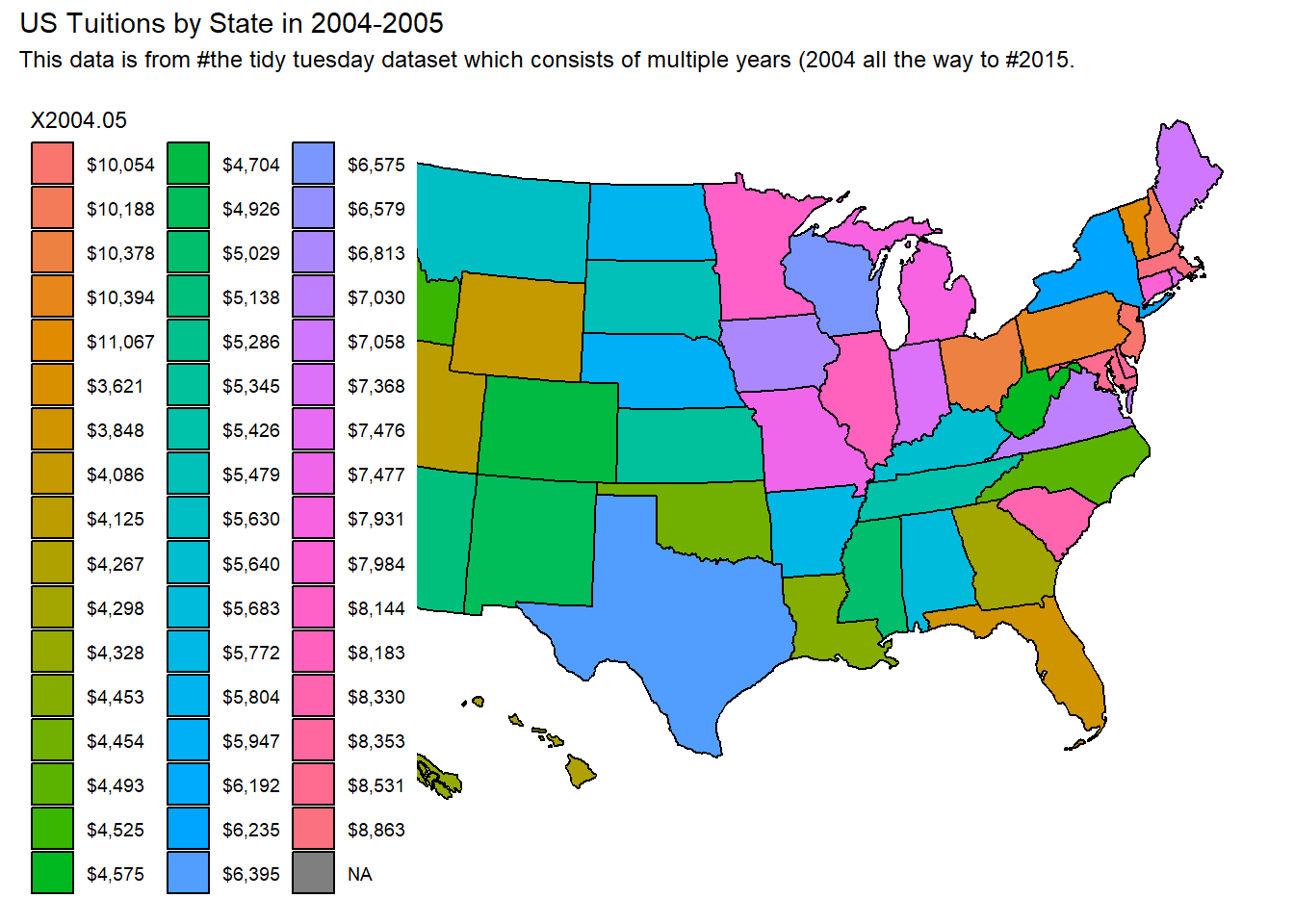
usmap::plot_usmap(data = avg_us_tuition, values ="X2004.05") +labs(title ="US Tuitions by State in 2004-2005", subtitle ="This data is from the tidy tuesday dataset which consists of multiple years (2004 all the way to 2015.") +scale_color_continuous(type ="gradient")
Image of visualization due to github errors with packages
Reflection for today’s visualizations
Some takeaways after learning to plot a US Map graph:
The package usmap, is very handy for visualizations referencing states and comes with ggplot2 functionality (allowing you to use ggplot functions).
The package requires a “state” column (case sensitive) in order to recognize a dataframe and build off of it.
Currently the visualization isn’t great because each state has its own specific key. This makes the colors all over the place.
Discrete vs Continuous
R is treating the avg US tuition as a discrete variable and I don’t want that! I’ll need to make it continous.
Visualizations 2 & 3, Plus next steps
Next, I should set a proper color scale for the various tuition costs to make the graph a lot cleaner. As you can see, it doesn’t actually graph the average US tuition on a scale, so I will need to modify the values slightly to do this.
That means I will
1. Need to pivot some values around (I want the year as values not variable)
2. Need to apply continuous data for the avg. tuition so that I can use the scale.
I also decided to reformat the years just to have the specific start year (rathar than 2004-2005 the new format would be 2004). Below you can find the r code doing that.
library(tidyverse)library(ggplot2)library(janitor)avg_us_tuition <-read.csv("datasets/us_avg_tuition.csv")#renamed column from "State" to "state" as usmaps won't recognize the column otherwise.avg_us_tuition <- avg_us_tuition |>rename(state ="State")head(avg_us_tuition)
#pivot dataframe (Year is a value and not a variable)pivot_avg_us_tuition <- avg_us_tuition |>pivot_longer(cols =!state,names_to ="year",values_to ="avg_tuition_cost" )#removing comma (not sure if necessary)pivot_avg_us_tuition$avg_tuition_cost <-str_replace_all(pivot_avg_us_tuition$avg_tuition_cost, ",", "")#regex to mutate the values of the year to be more readable (instead of X2004-05 rename it to 2004).#and then make sure to save the resultpivot_avg_us_tuition <- pivot_avg_us_tuition |>mutate(year =str_extract(year, "\\d\\d\\d\\d"),avg_tuition_cost =str_extract(avg_tuition_cost, "(?<=\\$).*") #?<= is a look behind regex function (in this case is "$") )head(pivot_avg_us_tuition)
pivot_avg_us_tuition[3] <-lapply(pivot_avg_us_tuition[3], as.numeric)pivot_avg_us_tuition[2] <-lapply(pivot_avg_us_tuition[2], as.numeric)#grab the entries starting from year 2004 (to 2005)us_tuition_2004 <- pivot_avg_us_tuition |>filter(year =="2004") head(us_tuition_2004)
# A tibble: 6 × 3
  state       year avg_tuition_cost
  <chr>      <dbl>            <dbl>
1 Alabama     2004             5683
2 Alaska      2004             4328
3 Arizona     2004             5138
4 Arkansas    2004             5772
5 California  2004             5286
6 Colorado    2004             4704
Now that the dataset looks tidied up, next I will try to plot the usmap again:
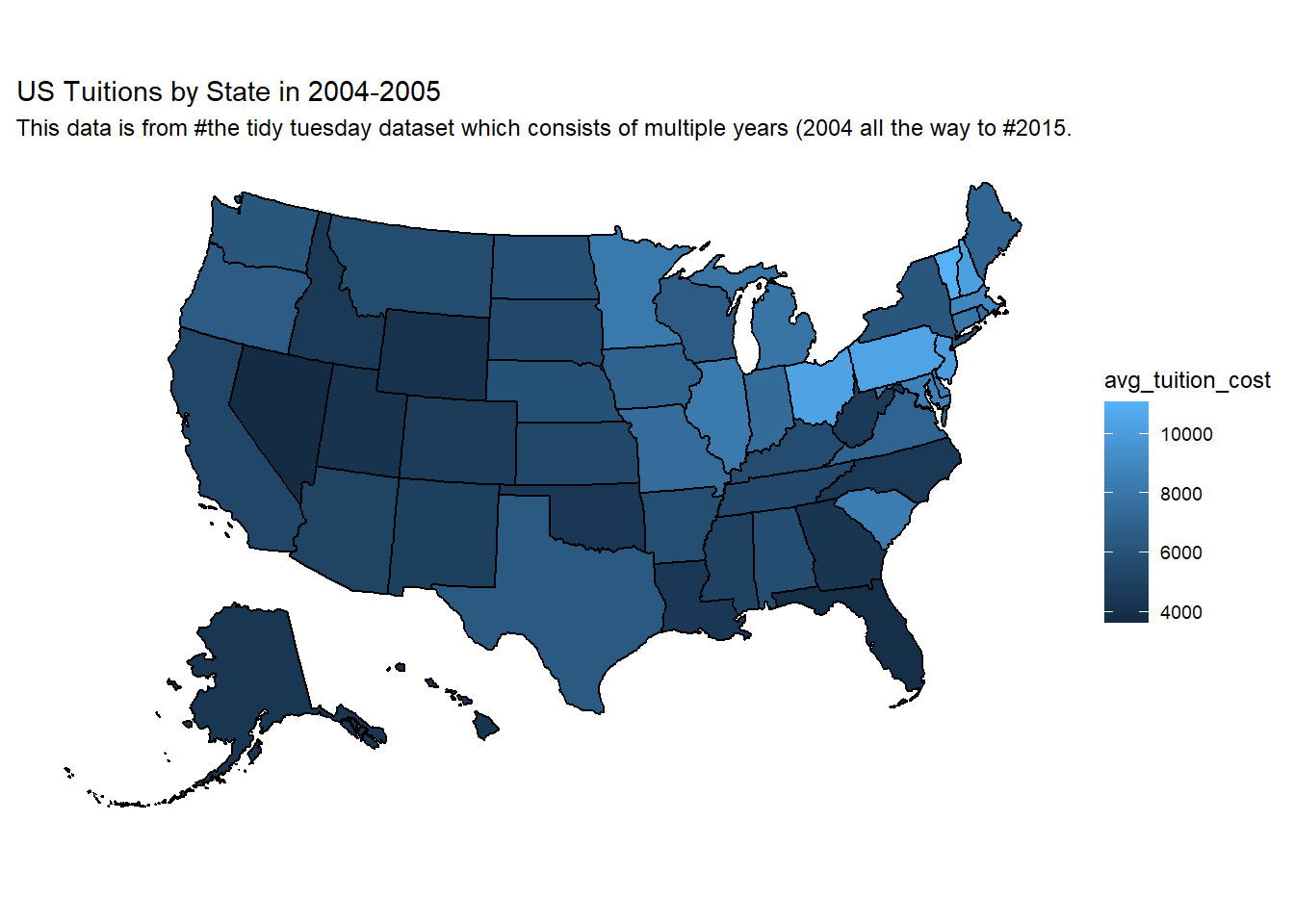
#Making a visualization with usmap using a continuous scale:usmap::plot_usmap(data = us_tuition_2004, values ="avg_tuition_cost") +labs(title ="US Tuitions by State in 2004-2005", subtitle ="This data is from the tidy tuesday dataset which consists of multiple years (2004 all the way to 2015.") +scale_color_continuous(type ="gradient", label = scales::comma) +theme(legend.position ="right")
Image of visualization due to github errors with packages
Looks great now! 😃
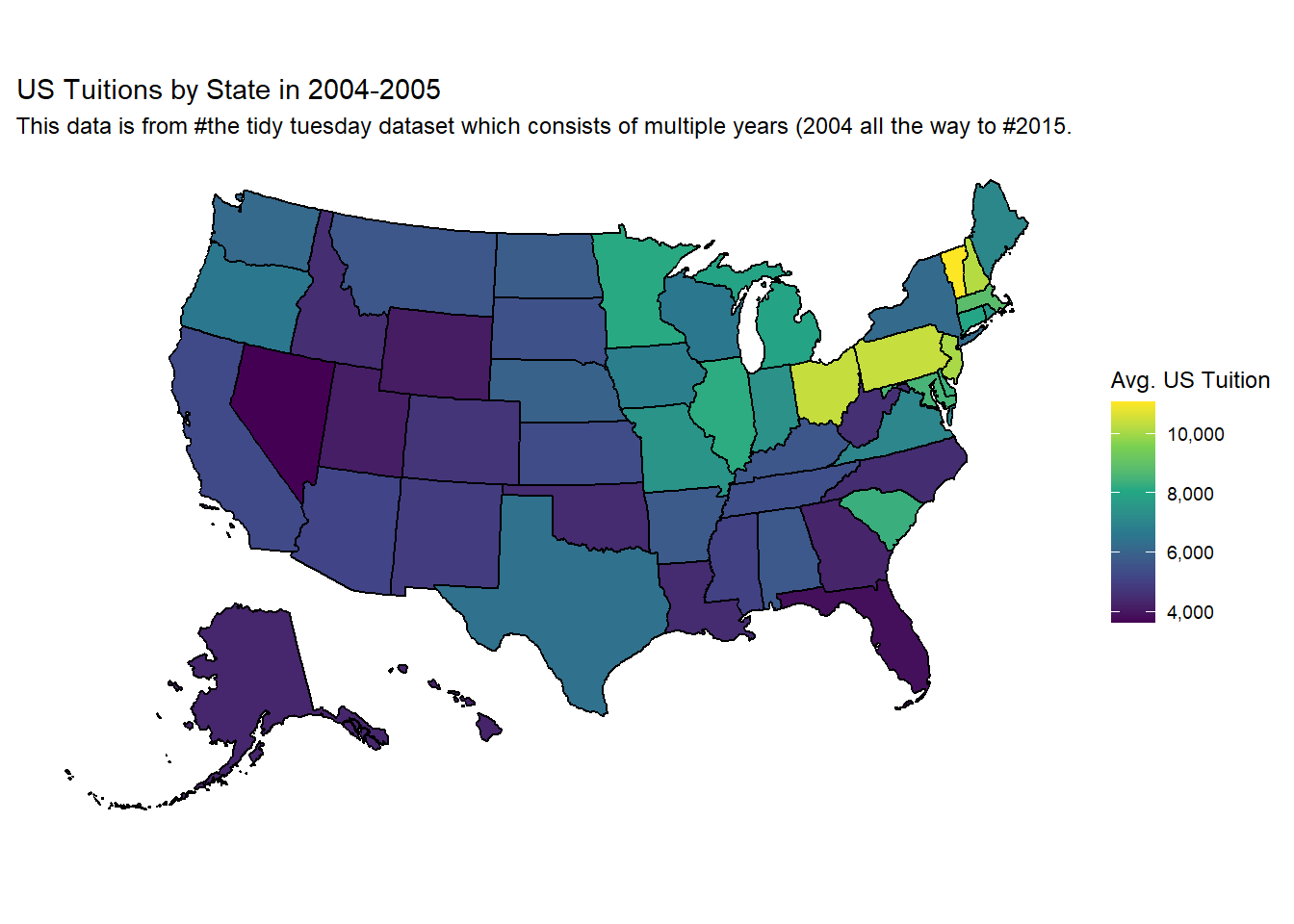
I also learned about a colorblind friendly scale which I tried to apply in a similar visualization and I liked it a bit more than the simple gradient I have above.
#Making a visualization with usmap with viridis (colorblind friendly) continuous scale: usmap::plot_usmap(data = us_tuition_2004, values ="avg_tuition_cost") +labs(title ="US Tuitions by State in 2004-2005", subtitle ="This data is from the tidy tuesday dataset which consists of multiple years") +scale_fill_viridis_c(name ="Avg. US Tuition", label = scales::comma) +theme(legend.position ="right")
Image of visualization due to github errors with packages
Reflection for today’s visualizations
These 2 visualizations were quite challenging to reach too. I think that’s due to some things I didn’t realize before working towards them.
For one, I didn’t think much about the avg tuition being a discrete variable which unsurprisingly would cause trouble with scale for the visualization. Once I realized that and properly adjust the variable to be continuous, that problem was fixed!
The other issue I had was from working on tidying up the data, after recently learning about pivoting. I recognize though the usefulness of pivoting as earlier I didn’t even think about how the years would actually be more appropriate as values in a cell rather than as a column as a variable.
I also had to look up a lot of the functions for tidying up data. I’m currently taking some time to get understand the functions and arguments I used for the visualizations! 📘📘📘 (some of those functions include scale_fill_viridis_c for a more colorblind friendly scale, using scales::comma to add commas to the scale values and of course, the usmap package for visualizations with a map)
Next steps #2
What do I plan on doing for the last visualization?
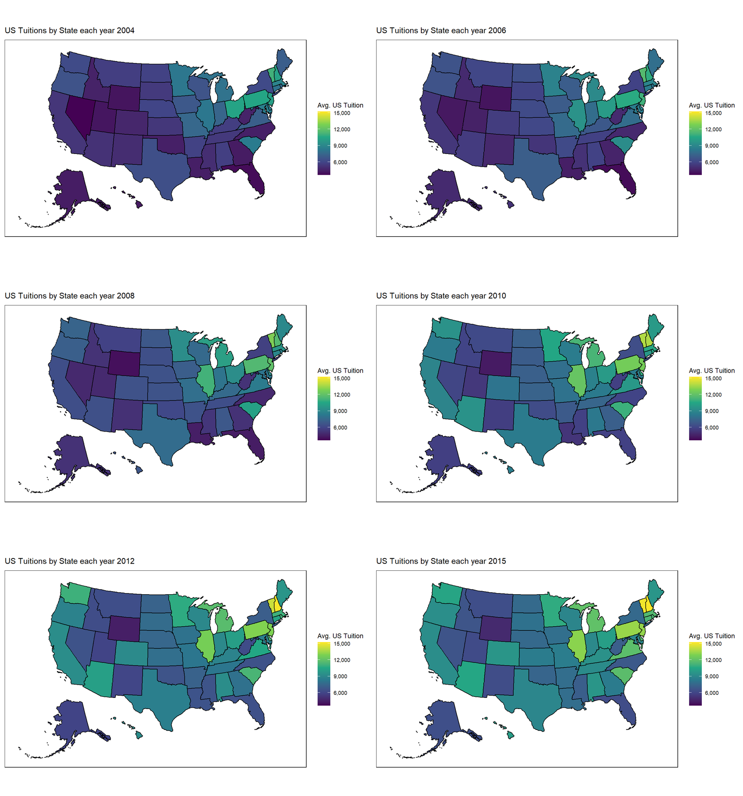
I saw another person, Jen Richmond create some awesome usmap visualizations as well! Especially interesting is the graph at the bottom of the post, which consists of a really awesome gif visualization capturing the yearly change of nurses hourly wages and I’d like to apply that to my current visualization too! So, up next I’ll be trying to learn how to do that from her post and take some time reflecting and detailing the process, and what I learned from doing it.
So far what I’ve learned about making an animated gif graph over time from Jen’s post is that the functionality is done easily through gganimate.
library(gganimate)library(ggplot2)library(ggeasy)#Almost the same as previous, except we will be transitioning the label (to show that the years are changing)plot <- usmap::plot_usmap(data = pivot_avg_us_tuition, values ="avg_tuition_cost") +scale_fill_viridis_c(name ="Avg. US Tuition", label = scales::comma) +easy_move_legend(to =c("right")) +#these following 2 lines from Jen's post is to stylize the graph a bittheme(panel.background =element_rect(colour ="black"))#note how the resulting visualization has a black border and the position of the legend is to the right.#modify labels to transition (based on the year)transition <- plot +labs(title ="US Tuitions by State each year {as.integer(frame_time)}") +transition_time(year)#then we animate the plot gif <-animate(transition, fps=8, renderer =gifski_renderer())#viewing the gifgif#And then finally, saving the file as a .gifanim_save(filename ="map_avg_tuition.gif")